Synopsis
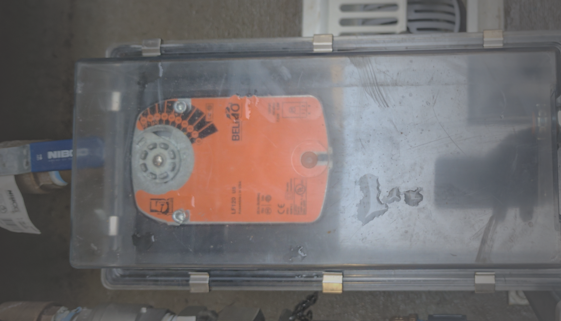
Any real-world process is typically subject to system upsets. Controlling cooling towers can be far more challenging than it would appear. It seems that every time you look the other way, a ball valve which should be open gets closed, a strainer gets clogged, or a solenoid valve gets stuck. With so many points of contact and “gears” spinning, something inevitably goes wrong. I have been working for some time now in simulating system failure modes. In these real-world applications, it is nice to know what the cost of certain system failures are without having to foot the bill.
The interactive chart below allows you to adjust a series of sliders, which represent your unique process. The rest is mathematical approximation. This simulation compares scale accumulation between an online controller and offline controller in the event of a blow down valve being stuck in the closed state. Murphy’s Law of Cooling is powered by a useful tool called “high charts”, and this use is intended for educational purposes.
Nutshell
For those of you intricately curious about the calculations used in the back end, scroll to the “Detailed” section. In a nutshell, the simulator takes in the make-up water parameters: conductivity, alkalinity, and hardness. The pH value is inferred based on alkalinity. Initial system concentration is based on make-up parameters and cycle of concentration set point. Once the assumed valve failure occurs, the rate of “cycling up” is based on: the system volume, evaporation rate (concentrating solids), and drift (dispersing solids). From that point, the tool deduces cycles and LSI value with respect to time. The LSI tendency will give us our “scale” or “corrosive” tendency. For now, the tool only works to showcase scaling nature water and will simulate scale deposition in a chiller and begin calculating the opportunity cost.
The comparison is between an online controller and an offline controller and illustrates differences based on resolution time. The resolution time assumes that offline system failures resolve at 50% of the service interval frequency while an online device is resolved 24 hours after the system is a full cycle above the desired set point. Scale accumulation is based on these system parameters and prorated for inhibitor effectivity. Scale thickness determines the efficiency loss of a system and the associative cost. Note that this is a simulation; there are a lot of mathematical approximations which are made to generate these numbers. I hope you find this visual representation useful.
Detailed
If you are reading this section, you are either really curious, or you do not agree with the graph. Below, you will find all of my calculations and assumptions in a very methodical and mathematical approach. As mentioned previously, this is an approximation. There are no “hard rules” for some of the approximations I have made. At a certain point, to really dial in the calculation, you would need to factor in the actual physical geometry of the chiller, the number of tubes, passes, diameter, temperature gradient, through-put, and more!
Cycling Up!
Three factors go into calculating the cycles of concentration in the simulator: system cycle inertia, pure water lost to evaporation, and drift. System cycle inertia is the system volume multiplied by concentrated cycles. Then, when pure water leaves the system, due to evaporation, the water will be replaced by make-up water concentrating the solids. Drift, or any water which exits the recirculation loop, would effectively blow-down and subtract the concentrated solids.
\( Cycles_{Concentrated} = {(System\ Volume * Concentrated\ Cycles) + (Evaporation * Make\ Up\ Cycles) – (Drift * Concentrated\ Cycles) \over System\ Volume}\)
\( Evaporation = {Q {BTU \over hr} * 24 {hr \over day} * F_{factor} \over 1040 {BTU \over lb} * 8.345 {lb \over Gal}}\)
\( F_{factor} = 0.8\)
\( Q {BTU \over hr} = System\ tons * Load\ \% * 12,000 {BTU \over hr}\)
\( Load\ \% = Typical\ System\ Load * Efficiency\ (drops\ when\ scale\ accumulates)\)
\( Drift {Gal \over hr} = F_d * Recirculation\ Rate {Gal \over hr}\)
\( F_d = Drift\ Factor\ (User\ Defined)\)
\( Recirculation\ Rate {Gal \over min} = 3 * System\ Tonnage \)
\( Recirculation\ Rate {Gal \over hr} = Recirculation\ Rate {Gal \over min} * 60 \)
How accurately are we calculating cycles of concentration? There are a few assumptions. Our “F factor” is fixed at 0.8, in reality it can range from 0.75-1.00 depending on environmental factors, mainly humidity. Load in this simulator is a fixed percentage value. Note that the actual system load would typically fluctuate. Additionally, the recirculation rate is assumed based on tonnage.
Langilier’s Saturation Index
This scale, and similar scales, helps indicate whether water has a more corrosive, balanced, or scaling tendency. It is a useful indicator of the “nature” of your process water.
$$LSI = pH_{Calculated} - pH_{s}$$
$$pH_{Calculated} = 1.718 * \log{(Alkalinity * Cylces_{Concentrated})} + 4.133$$
$$pH_s = (9.3 + A + B) - (C + D)$$
$$A = {\log{(TDS)}-1 \over 10}$$
$$TDS = Make\ Up {uS \over cm} * Cylces_{Concentrated} * 0.64$$
$$B = (-13.12*\log {(Temp_k)}+34.55)$$
$$Temp_k = {5 \over 9} * (Temp_F + 459.67)$$
$$C = \log{(Calcium\ Make\ Up\ PPM * Cycles_{Concentrated})} - 0.4$$
$$D = \log{(Alkalinity\ Make\ Up\ PPM * Cycles_{Concentrated})}$$
What is our stack up? Concentrated cycles are a calculated value. This calculated value has aforementioned errors and is used as a coefficient in the LSI calculation. The pH value is approximated based off alkalinity. Also, I convert uS/cm into TDS using 0.64 as a coefficient, which is an “accepted” conversion but not always a precise or accurate conversion. Also, this tool simulates scale accumulation. Scale formation would technically reduce the calcium in the process since it would “drop out” of suspension. Calculating the reduction of suspended calcium became very involved. Knowing the exact rate of nucleation is largely a guess as too many system parameters are involved in the process, and it depends on a lot of surface area mapped to heat gradients and inhibitors that innately interrupt the nature of this process.
Scale Thickness
This is by far the most approximated measurement in the simulation tool, yet it is pivotal at relaying the point. During my research phase of this piece, I read a number of very long-winded papers about controlled experiments which had scale formation about an interesting and new “index” to help quantify the rate in which scale accumulates. There were large numerical deltas between each paper I read, so I decided, for illustration purposes, to design a function of my own as a “feeler” for scale accumulation. All the research papers I read agreed that developing an initial scale film takes a little time. Once a good foundation has been set, scale formation occurs rapidly. When the scale becomes obtrusive enough, the flow of water will chisel away at the scale almost as fast as it settles, plateauing the growth. Scale inhibitors complicate the math. These chemicals delay the process of scale formation in various ways. They do not halt scale formation completely, but they “modulate” the rate of scale accumulation.
$$Scale\ Thickness = Arctan\ Coefficient * (LSI - Effectivity) * 30$$
$$Arctan\ Coefficient = \arctan {({Time\ Since\ Valve\ Failure \over (5 * Delay)} - Delay)} + \arctan {(Delay)}$$
$$Delay = 5 + 5 * Inhibitor\ Effectivity$$
$$Effectivity = 2 * Inhibitor\ Effectivity$$
How accurate is the Scale Thickness approximation? It could be dead on! My coefficients are based on results in controlled experiments; however, this function was created from scratch based on only a little experimental data. The Arctan function simply resembles the way scale typically accrues. I added in some parameters to help shift and morph the function based on LSI and Inhibitor. Unfortunately, LSI is not an index which can project rate of scale, only its tendency. Delay helps shift and stretch the slope of the function to postpone and reduce scaling tendency with inhibitor effectivity. The equation above is a great illustrative tool, but academically, a work in progress.
Cost
Opportunity cost! This is the main reason I started this thought experiment; how does response time impact the end user on their efficiencies?
$$Energy\ Loss = Efficiency\ Coefficient * Cost\ of\ Power * Load * System\ Tonnage * 3.5$$
$$Efficiency\ Coefficient = 1 - e^{(-0.009*Scale\ Thickness)}$$
Technically, the calculation on the back end is a Riemann sum of the total efficiency loss. Bear in mind that the tool only shows the current opportunity loss from scale formation. After the valve is fixed, the scale is still causing inefficiencies. This effect, compounded over time, can amount to astronomical values.
Conclusion
Thank you for reading this far, I hope you found this simulation useful. If you have suggestions on how to modify this tool to add more value, please do not hesitate to reach out to me. Additionally, this is completely open source. If you would like to use this tool, modify it, or improve it, you are welcome to contribute to the greater good. I tried being relatively detailed in my code comments.


